Just-In-Time and Lead-Time Reduction: A Retail Operator’s Guide to Cutting Inventory Without Cutting Service
How lead time drives inventory arithmetically, the eight levers ranked by cash impact, when pure JIT fails, and the segmented hybrid model most sophisticated retailers converge on.
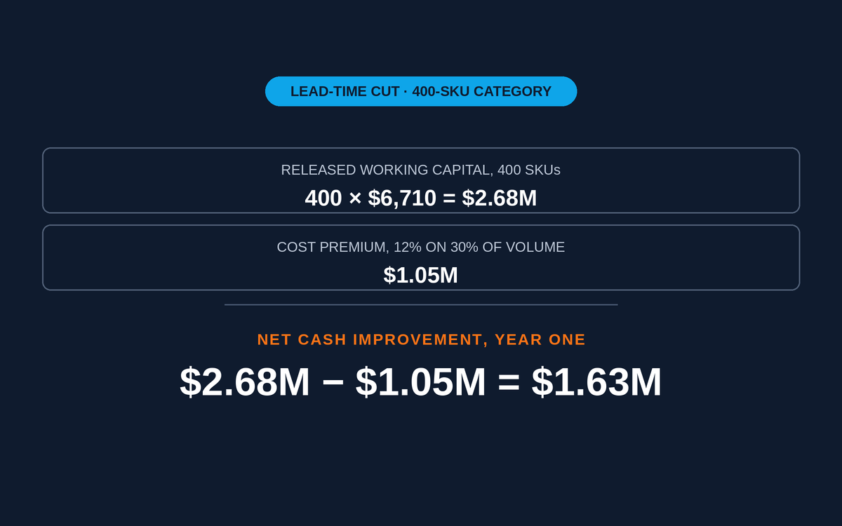
Table of contents+
Through most of the 2010s, retail operations orthodoxy said the same thing every quarter: cut inventory, shorten lead time, run leaner, run faster. Toyota’s just-in-time philosophy had migrated fully into retail buying rooms. Working capital targets tightened year after year. Grocery chains ran daily replenishment on 80 percent of ambient SKUs. Fast-fashion players squeezed apparel design-to-shelf cycles below 21 days. The industry consensus was that inventory was a symptom of forecasting failure, and every day of lead time was a day of cash trapped between the supplier’s dock and the customer’s hand.
Then 2020 rewrote the arithmetic in eighteen months. Ocean freight rates went 4x. Ex-China lead times stretched from 45 days to 120. Retailers that had run at 2.5 weeks of forward cover on offshore SKUs found themselves stocked out for entire selling seasons while inventory floated in Long Beach. The pendulum swung hard toward buffer stock, and by 2022 many operators had over-corrected in the opposite direction: category-level inventory 40 percent above pre-pandemic levels, inventory turnover down two turns, and category managers unable to articulate why the buffer existed on any specific SKU. The right answer sits in neither era. Modern retail operations blend JIT for the categories where it actually works with disciplined lead-time reduction on the categories where it does not, and buffer only the specific SKUs that mathematically justify the carrying cost. What follows is that discipline in operator terms: how lead time drives inventory arithmetically, the eight levers ranked by cash impact, when pure JIT fails, and the hybrid model that most sophisticated retailers now run.
JIT and lead-time reduction as one lever
JIT and lead-time reduction are frequently discussed as two separate topics. In practice they are two ends of the same lever. JIT is a replenishment posture: order inventory to arrive right as demand pulls it, hold as little as possible in between. Lead-time reduction is the enabling condition: the shorter the supplier can deliver, the closer the operator can run to JIT without losing service. A retailer cannot commit to JIT on any SKU whose lead time is unreliable, and there is no point in reducing lead time on a SKU the operator has no intention of running lean.
The connection is arithmetic, not philosophical. Every day of average lead time raises the minimum on-hand inventory needed to hold a given service level. Every unit of lead-time variability raises it further. Compress either input, and the safety-stock formula releases working capital automatically. This is why lead-time reduction usually pays back in six to twelve months even when the unit cost of the shorter option is meaningfully higher: the working capital release, the markdown risk avoided, and the responsiveness gained on trend shifts almost always outweigh the incremental cost per unit.
The formula that links them
The reorder-point formula makes the connection concrete.
Reorder Point = (Average Daily Demand × Lead Time) + Safety Stock
Safety Stock = Z × √( (LT × σD²) + (D² × σLT²) )
Two inputs drive the entire result: average lead time (LT) and lead-time variability (σLT). Shortening average lead time cuts the cycle-stock portion of on-hand inventory linearly. Shortening lead-time variability cuts the safety-stock portion under the square root. In most offshore-sourced retail categories, the σLT term dominates the σD (demand variability) term inside the safety-stock formula, which is why supplier reliability improvements usually deliver larger inventory reductions than demand-forecasting improvements at the same investment level. The Safety Stock Calculator and Reorder Point Calculator do the arithmetic on any specific SKU.
Worked example: cutting 20 days on a specialty apparel SKU
A specialty apparel retailer sources a wool sweater from an offshore vendor. Current state: average daily demand 12 units, average lead time 60 days, lead-time standard deviation 14 days, demand standard deviation 3 units, service-level target 95 percent (Z = 1.65). The safety-stock formula gives approximately 279 units of safety stock. Cycle stock at reorder = 12 × 60 = 720 units. Reorder point = 999 units. Average on-hand across the cycle roughly 640 units. At a landed cost of $45 per unit, that is $28,800 of working capital tied up in one SKU.
Now compress lead time. The retailer moves 30 percent of the volume to a domestic nearshore supplier at a 12 percent unit-cost premium ($50.40 per unit). Lead time on the domestic portion drops to 18 days with a standard deviation of 4 days. Blend the two sources at 70 percent offshore, 30 percent domestic. Blended average lead time: 47.4 days. Blended σLT: approximately 11.2 days. The safety-stock formula now gives roughly 210 units. Reorder point drops to 779 units. Average on-hand drops to about 480 units. Working capital tied up: $22,090. Working capital released: $6,710 per SKU per cycle.
Across 400 SKUs in the category, that is $2.68M of released working capital against an incremental annual COGS increase of roughly $1.05M (the 12 percent premium on 30 percent of the volume). Net cash improvement in year one: $1.63M, before counting reduced markdown risk on the domestic-sourced portion, which typically adds another 2 to 4 percentage points of gross margin retention.
The domestic premium looks expensive at the unit-cost level. Priced against released working capital plus avoided markdown, it usually pays back inside 18 months on any category with real trend risk.
The eight lead-time levers, ranked by cash impact
Eight levers reduce lead time in retail supply chains. They are ordered here by typical cash impact per dollar of program investment, not by how frequently retailers talk about them.
1. Measure actual end-to-end lead time first
Most retailers know supplier-quoted lead time but not actual end-to-end lead time, which includes PO processing, supplier queue, manufacturing, transit, customs, receiving and putaway. The difference is routinely 30 to 50 percent. A quoted 45-day supplier is often a 62-day supplier once every internal handoff is measured. This costs nothing to fix and often finds two to three weeks of hidden lead time inside the retailer’s own processes.
2. Tighten inbound discipline
PO processing, dock scheduling, receiving accuracy and putaway routinely add 3 to 7 days that no operator tracks. These are internal, controllable, and free to fix. Move PO issuance to a same-day cadence, book vendor delivery appointments 5 days ahead, and cut receiving-to-putaway lag to under 24 hours. This is the cheapest source of lead-time reduction available, and it usually shows up on the OTIF scorecard within one quarter. See the OTIF Calculator for scoring the vendor half of the same measurement.
3. Switch supplier communication to EDI
Email-based PO processes lose 3 to 5 days versus EDI. Most modern ERPs support EDI integration with major suppliers. Technology cost is small, integration timeline is 8 to 12 weeks per major supplier, and the lead-time savings persist forever. On high-frequency replenishment SKUs, the compounding effect is meaningful.
4. Split sourcing across offshore and near-shore
Source 60 to 80 percent of a category from the lowest-cost offshore option and 20 to 40 percent from a domestic or near-shore option. The domestic source runs as a chase strategy: when an item is selling, replenish in 2 to 3 weeks instead of 8 to 12. The blended unit cost rises modestly, but working capital falls more than the cost premium and markdown exposure drops sharply on the trending SKUs.
5. Supplier collaboration and VMI
Negotiate vendor-managed inventory or collaborative planning where the supplier sees your forecast in real time. What looks like supplier slowness is often demand volatility hidden by long planning cycles. VMI programs typically compress lead time 20 to 35 percent and cut supplier-side variability by more than half. See the VMI guide for how the operating model works in practice.
6. Nearshore strategic categories
For the top-25 SKUs by revenue in each category, evaluate a full nearshore move. The unit-cost premium (10 to 25 percent) usually pays back within 18 months once the working-capital release, avoided markdowns and improved sell-through on trend items are all counted. This is the most capital-intensive lever and belongs late in the sequence.
7. Transit optimization
Ocean expedited service, faster customs brokerage and direct-routing arrangements can shave 5 to 8 days off long-haul lead times at 20 to 40 percent of the cost of switching to air freight. Air freight remains justified only on stockout-sensitive high-margin SKUs where the gross-profit-dollar cost of a stockout exceeds the freight premium.
8. Safety lead time, used sparingly
Adding a time buffer to expected lead time protects service on critical SKUs. Use it only where variability is genuinely irreducible and only after the seven levers above have been exhausted. Safety lead time hides process problems if applied as a default, and every retailer who uses it broadly ends up with silent lead-time creep.
When pure JIT fails
Pure JIT breaks under four specific conditions. Recognize the pattern early or the working-capital advantage of JIT gets consumed by service-level failures.
Failure 1: Offshore sourcing on unstable freight lanes. Any SKU with ocean-shipped lead times above 45 days should not be run on pure JIT. The variance in the σLT term makes the safety-stock formula demand more buffer than the JIT posture is willing to hold, and stockouts follow within one shock cycle.
Failure 2: Demand volatility above 25 percent CoV. When demand CoV (coefficient of variation) exceeds 25 percent, the reorder point math requires either substantial safety stock or unrealistic forecast accuracy. JIT wants neither. Fashion, seasonal categories and promotion-driven SKUs typically live above this threshold and should not be on JIT regardless of lead time.
Failure 3: Single-source supplier concentration. A supplier at 100 percent of a SKU’s volume creates a single point of failure that JIT amplifies. The 2020 pandemic taught this lesson at industry scale. Dual-source the top-quartile SKUs by revenue as an absolute rule.
Failure 4: Weak demand signal to the supplier. If the supplier cannot see your forecast, they build their own buffer against your unpredictability, and their internal lead time expands accordingly. Fix by moving to VMI or shared-forecast collaboration before extending JIT to any new category.
The segmented hybrid model most retailers now run
Most sophisticated retailers converge on a segmented hybrid model. Four buckets, four different inventory postures.
Bucket A: Fast-moving, short-lead-time, stable-demand SKUs (grocery ambient, apparel basics with domestic replenishment). Near-JIT. Days of forward cover held to 5 to 10.
Bucket B: Fast-moving, longer-lead-time SKUs. Traditional reorder-point discipline with safety stock sized against demand variability. Days of forward cover 20 to 45.
Bucket C: Slow-moving, long-lead-time, seasonal SKUs. Buy-to-forecast model with markdown budget planned in. Cover measured by season, not weeks.
Bucket D: Strategic SKUs where stockouts are catastrophic (private-label anchors, service SKUs that draw traffic). Strategic safety stock funded explicitly as an insurance policy, held at higher cover than the math alone would suggest. See the private label strategy guide for how anchor SKU economics interact with buffer decisions.
The discipline is not choosing between JIT and buffer, it is running the segmentation cleanly and revisiting the segment assignments quarterly. A grocery-scale operator might run 60 percent of SKUs in Bucket A, 25 percent in Bucket B, 12 percent in Bucket C and 3 percent in Bucket D. A specialty apparel operator might run 15 percent, 30 percent, 50 percent, 5 percent. Both are correct answers to their respective category economics.
The takeaway
Lead time and inventory are two sides of the same working-capital equation. Every day and every unit of lead-time variability trapped in the supply chain funds nothing and earns nothing. The eight levers above attack that trapped capital in ranked order of cash return per program dollar. Start with the free ones (measurement, inbound discipline, EDI), move to structural ones (VMI, split sourcing) as the operating model matures, and only reach for capital-intensive changes (full nearshoring, air freight) once the earlier levers have been exhausted. Pair the lead-time attack with a disciplined JIT-versus-buffer segmentation so the working-capital release from shorter lead times does not evaporate into unnecessary safety stock elsewhere. Retailers that get both halves right typically run 20 to 35 percent lower category inventory at the same service level, one to two turns higher on category inventory turnover, and materially lower markdown exposure on trend-driven categories. The two disciplines pay each other’s rent.
Frequently Asked Questions
How much inventory does one day of lead-time reduction typically release?+
As a rough field rule, each day of average lead-time reduction cuts on-hand inventory by roughly 1 to 2 percent at the same service level, and each day of lead-time variability reduction cuts safety stock by 3 to 5 percent. The variance reduction is worth more per day than the mean reduction. That is why supplier reliability investments usually beat pure speed investments dollar for dollar.
Which lead-time lever should retailers start with?+
Measurement. Almost every retailer discovers 2 to 3 weeks of unmeasured internal lead time (PO processing, dock scheduling, putaway lag) the first time they map end-to-end lead time honestly. That week of savings costs nothing and is invisible until it is measured. See the OTIF Calculator for a starting scorecard on the supplier half.
Is JIT still relevant after the 2020 to 2022 supply shocks?+
Yes, in the categories where lead time is short and reliable to begin with. Grocery ambient, domestic apparel basics, and domestically-sourced private label all still run on near-JIT successfully in 2026. Pure JIT on unstable offshore lanes has been permanently retired by most operators, and correctly so.
What is the difference between safety stock and safety lead time?+
Safety stock is buffer inventory sized to protect against demand variability during the lead-time window. Safety lead time is a time buffer added to expected lead time to protect against lead-time variability itself. Most operators use safety stock as the default and only add safety lead time on specific SKUs where lead-time variance is unusually high and irreducible.
Does nearshoring actually pay back given the unit-cost premium?+
On strategic SKUs, usually within 18 months. The math has to include the released working capital, avoided markdowns on trend-sensitive items, and the customer-experience gain of higher fill rates. On commodity SKUs with stable long-cycle demand, nearshoring often does not pay back. The decision is SKU-level, not category-level, which is why blanket nearshoring initiatives frequently disappoint the finance team.
How much lead time can EDI actually save?+
Typically 3 to 5 days per PO cycle across email-driven supplier processes. EDI eliminates the manual data-entry loop, the confirmation-email round trips, and most PO error-correction traffic. On high-frequency replenishment SKUs, 3 to 5 days per cycle compounds into meaningful annual inventory reduction. The upfront integration cost is usually recovered within one to two quarters.
Should lead-time reduction come out of the supply chain budget or the merchandising budget?+
Split ownership. Merchandising owns the sourcing-choice trade-offs (nearshore versus offshore, split sourcing, supplier selection). Supply chain owns the operational levers (measurement, inbound discipline, EDI, transit optimization). The programs that succeed have a single executive sponsor holding both budgets accountable to the same working-capital release target.
What breaks first when a retailer overshoots into too much buffer stock?+
Category gross margin and GMROI. Excess buffer drives markdowns as inventory ages past its selling window, and GMROI collapses because the margin-per-inventory-dollar ratio falls on both numerator and denominator at the same time. When GMROI trends down two quarters in a row without a corresponding pricing or cost shock, buffer inflation is usually the reason. See the DIO Calculator for the fastest early-warning signal.
How often should the JIT-versus-buffer segmentation be revisited?+
Quarterly at minimum, and always after a material supply-side shock. SKU velocity shifts, supplier lead times drift, and demand volatility profiles change faster than most retailers refresh their inventory policies. Retailers running annual reviews find their bucket assignments meaningfully stale by month nine. Quarterly reviews take a working session per category and pay for themselves in avoided stockouts and released capital.
What is the fastest way to reduce lead-time variability specifically?+
Consolidate volume with the top-quartile of the supplier base. Variability is dominated by capacity contention at the supplier’s factory. Suppliers who see you as a top-5 customer prioritize your production runs and hold your slot when their queue tightens. Suppliers who see you as a top-40 customer let your PO drift when capacity gets short. Volume consolidation is the highest-impact variability lever available, and it is free.
Related Calculators
Try the math from this guide with our free tools.
Reorder Point Calculator
Set the trigger level that fires the next PO for an SKU. Reorder point combines expected demand during lead time with a buffer for the weeks that run hot. Get either half wrong and you either stock out or bury cash on the shelf. Outputs are the ROP itself, the lead-time demand behind it, the buffer as a percent of expected demand, and the days of supply that ROP represents at current sales velocity.
Open calculator
Safety Stock Calculator
Size the buffer that keeps shelves stocked when demand spikes or the truck runs late. Enter a target service level, your demand history, and lead time to get the exact number of units to hold above expected demand. No more guessing with "two extra weeks of supply."
Open calculator
Inventory Turnover Calculator
Measure how many times a year your average inventory sells through and gets replaced. The single most consequential operational KPI in retail. It connects buying decisions, warehouse cash, markdown risk, and finance targets into one number. The turn ratio arrives converted into days and weeks of supply, together with the working capital a one-turn improvement would release. Departments that carry stock at retail value rather than cost usually track it with a retail inventory method tracking template, which produces the same average-inventory figure this calculator needs.
Open calculator
EOQ Calculator
Find the order size that minimizes what you spend keeping an SKU stocked. Small orders push order cost up. Big orders push carrying cost up. EOQ finds the point where the two curves cross so you stop paying more than you have to, and it anchors every reorder point and safety stock decision downstream.
Open calculator
OTIF Calculator
OTIF is the single most widely used supplier scorecard metric in retail because it's binary and unforgiving by design: an order that arrives on time but short a case doesn't count, and an order that's complete but three days late doesn't count either. You end up with the OTIF percent and the distance from a 95 percent target. The distance is the part that starts the supplier conversation.
Open calculator
Days Inventory Outstanding Calculator
Convert your inventory position into a number finance actually reads: the average days of cash sitting on the warehouse floor. DIO is the same measurement as inventory turnover in days instead of a ratio, and it maps directly onto working capital, cash conversion cycle and reorder cadence. Four numbers come out: DIO, weeks of supply, implied turnover, and the cash a 10-day improvement would release.
Open calculator
Related Articles

Supply Chain KPI Guide: 12 Metrics That Matter for Retailers
A reference of the twelve supply chain metrics that actually drive availability, cost, and customer experience for retailers.

Drop-Shipping for Retailers: The Working-Capital-vs-Margin Trade
Drop-shipping trades margin for reduced inventory risk. The trade prices out well for long-tail SKUs and poorly for fast-turning A-class inventory. The decision framework and where the hidden costs sit.
Vendor Managed Inventory (VMI): Pros, Cons, and Setup Guide
Vendor managed inventory (VMI) for retailers: how it works, when it pays off, and how to set it up with key suppliers.
Explore Related Resources
Handpicked benchmarks, templates and guides to help you dig deeper.